How Accurate are VMT Estimates?

Link to article: https://stillwaterassociates.com/vmt-estimates/

October 15, 2019
By Gary Yowell

Estimating vehicle miles traveled (VMT) has important implications for analyzing and forecasting transportation fuel use and carbon dioxide CO₂ emissions. VMT estimates are frequently used as the foundation for transportation fuel use analyses and forecasts. This practice should be carefully examined, especially given the four widely varying VMT estimates found for the same historic period. Of all the factors used to evaluate and forecast transportation fuel use, VMT is the last factor to be determined and the least accurately known. VMT changes are sensitive and specific to fuel prices and indirectly to the economy. Properly prepared transportation forecast results are dominated by the VMT estimate applied, which is dominated by the fuel prices and subsequent economy conditions. This paper examines four VMT estimates, one of which is a new method I am developing which is uniquely based on U.S. EPA sales proportioned fuel economy values (link to Excel file download). I call it the Simple Forecast Method.

In California (and similarly the nation) there was an unprecedented $3.30 gasoline price increase from January 2002 through June of 2008. That price increase paired with the December 2007-June 2009 “Great Recession” created a short period of marked change in two of the indicators which affect VMT – fuel price and economic condition. Accurate VMT estimates should reflect these changes in real-time. How do current VMT estimation methods stand up to this unique opportunity to test and validate VMT estimates?

State Department of Transportation agencies use on-road vehicle measurements and proxy information to estimate statewide VMT for federal fuel tax allocations. For on-road derived VMT estimates, all vehicle traffic (both light- and heavy-duty) is included and used to inform the analysis. However, based on prior analyses, light-duty vehicles represent the vast majority (93%) of all VMT. As such, for simplicity, we exclude heavy-duty vehicles in this discussion.

The California Department of Transportation (Caltrans) uses its Highway Performance Monitoring System (HPMS) which includes 50-250 roadway meters operating three-to-four weekdays per week counting vehicles and applies vehicle fuel economy values and fuel sales data to create a combined estimate of VMT. This method has a common basis with other states reporting VMT to the Federal Highway Administration which is part of the basis used for federal fuel tax allocations. We will contrast the Caltrans VMT estimate with the California Air Resources Board (CARB) VMT estimate which is documented with the Emission Factors (EMFAC) model. We also compare the California Energy Commissions (CEC) VMT (Class-Based) estimate with the new Simple Forecast Method’s VMT estimate.

Figure 1 shows the four California VMT estimates mentioned above alongside total fuel sales. As can be seen, total fuel sales are aligned with the first four VMT years of the CEC VMT (Class-Based) estimate. This is because fuel prices and fuel economy trends prior to this time was relatively stable, especially compared to the turbulent times after 2003. Since at least 1950, statewide fuel sales and VMT has had a long growth history but both start their major decline after 2004, in response to significant fuel price increases. VMT generally follows the fuel sales volumes downward to 2011 until the economy strongly rebounds and pulls VMT upward. The 2005-2011 fuel sales decline was unprecedented for California which historically increased 275 million gallons annually from 1950 to 2004.

Figure 1. CARB, CEC, and Caltrans (HPMS) Estimated Total Statewide VMT Contrasted with a Simple Forecast Method and Total Fuel Sales

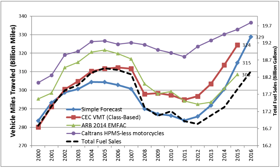
The 2007 VMT departure from total fuel sales is the consequence of consumers purchasing vehicles with higher fuel economies evident as early as 2004 relative to 1990-2003 vehicle purchases. Also note the 2010 bump in fuel sales which is due to California shifting from 5.7% to 10% ethanol blends starting 2010. All gasoline sold from 2010 had 1.45% lower energy, lowering all gasoline vehicles fuel economy and resulting in additional fuel sales. If not analytically corrected this fuel composition change would lead to a VMT increase error as shown by the CARB EMFAC 2010 VMT bump.

All VMT estimates generally follow the same trends yet there are significant differences between them. The estimates shown in Figure 1 differ by 25 and 30 billion miles (8% and 8.8%) for 2000 to 2016 respectively. We may never know which is the correct absolute VMT value, but we can gain insights by dividing the VMT estimates by the reported fuel sold to test the VMT accuracies. Figure 2 displays this calculation, yielding the effective fleet fuel economy in miles per gallon (mpg) for all vehicles, pickup trucks, and heavy-duty diesel vehicles.

Figure 2. Effective Fleet Fuel Economy Implied by VMT Estimates

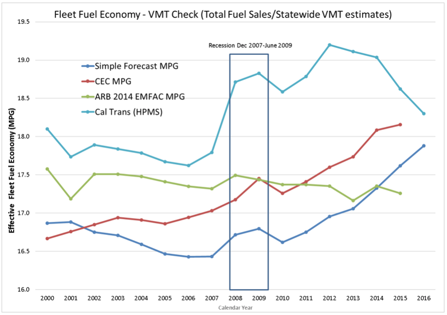
Note: Total Fuel Sales represents the volumes (and volume-equivalent displacements by alternative fuels) of gasoline, diesel, propane, natural gas, electricity, E-85 and hydrogen. Gas and diesel fuel sales volumes represent 99.6% of all fuel sold in 2016.

Let’s take a look at which of the four VMT estimates holds up the best over time by comparing their fleet mpg trends shown in Figure 3 and VMT vs total fuel sales trends.

Figure 3. EPA National Fuel Economy Trends Report

The Simple Forecast

The mpg estimate resulting from my Simple Forecast Method starts with a downward trend consistent with EPA’s fuel economy new vehicle sales trends. After 2005, the Simple Forecast method reverses direction and begins its ascent consistent with EPA’s light-duty vehicle fuel economy assent starting in 2005 and running through 2016. California’s effective fleet fuel economy lags a few years behind EPA’s new vehicle sales trend. It is reasonable for the California vehicle fleet of nearly 30 million vehicles to more gradually change direction given the fleet size compared to new vehicle sales fuel economy changes. Note: The 2007-2009 Recession interrupts the mpg trends; 2008 saw one billion gallons in reduced fuel sales and 2009 showed a 1.3-billion-gallon reduction when the trend had otherwise been upward.

Caltrans

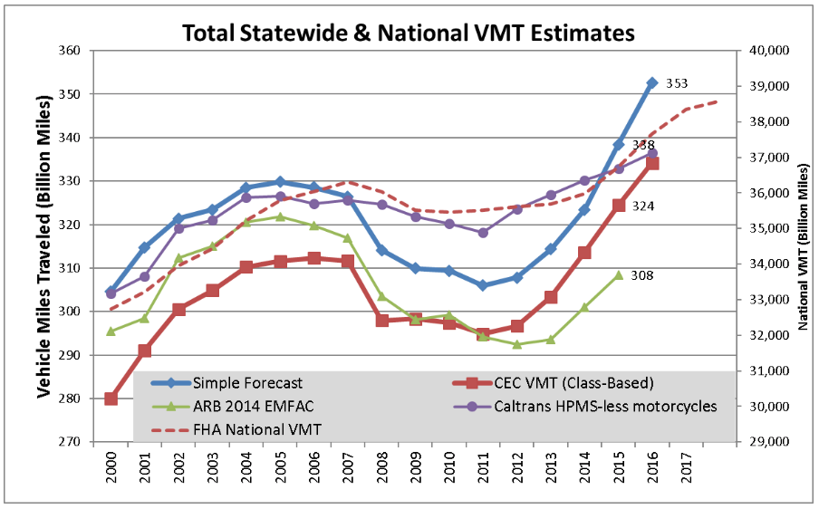
The HPMS-generated mpg trend appears to start out accurate and is more dynamic than the Simple Forecast mpg. It captures the Recession impacts, albeit apparently overestimating the mpg for the two years. This mpg overestimation is confirmed by referring to Figure 1 observing the gap between fuel sales and VMT. The Caltrans mpg trend incorrectly declines after 2012 in opposition to EPA’s mpg trends shown in Figure 3 and similarly observed California DMV new vehicle registrations fuel economy trends. Given that Caltrans’ California VMT estimates are similar to other states’ VMT methodologies, one might conclude that the Federal Highway Administration’s aggregate national VMT – which is compiled from these state-reported data – may be underestimating VMT or not recovering as fast after 2012 relative to the CEC or CARB estimates. This conclusion is supported by Figure 4 which includes the Federal Highway Administration National VMT estimate. Note the similar underreported recession impact on VMT in the 2008-2009 timeframe and reduced 2012-2017 VMT recovery similar to the Caltrans VMT estimate.

Figure 4. Contrasting National VMT with California VMT Estimates

CARB

The mpg trend generated using CARB’s EMFAC model generally trends downward over most years with a few exceptions when it should steadily increase from 2007-2016. It captures the first recession year in 2008 but misses the second year with more significant recession impacts and then effectively reduces mpg thereafter inconsistent with EPA fuel economy trends. Overall, CARB’s EMFAC shows a fundamental math logic error of setting the VMT equal to fuel sales for all years. See Figure 5 and note that the VMT correctly matches fuel sales for the first seven years but thereafter it does not increase over the Total Fuel Sales line suggesting no fuel economy improvements since 2000.

CEC

The CEC’s VMT estimate uses the identical vehicle populations and fuel volumes as the Simple Forecast Model. However, the CEC method evaluates VMT on a vehicle class-basis while the Simple Forecast Method uses actual vehicle fuel economy sales proportions. The differences between the CEC and Simple Method illustrate the range of VMT uncertainty depending on chosen methodology. EPA’s staff position is that the class-based method is significantly less accurate and is not recommend for use. This is because vehicle classes have fuel economy ranges of 63% compared to the EPA sales proportions have maximum ranges of 7%.

Conclusion:

All VMT estimates are derived from imperfect on-road measurements, vehicle populations, fuel economy, annual VMT decay estimates, and reported fuel sales. In short, all VMT estimates are based on proxy data of varying accuracy and confidence. Current VMT estimates have significant differences and considerable room for improvement. Before we can accurately forecast transportation fuel demand, we need to improve estimating past VMT. We should also be careful of the confidence we apply to VMT estimates, even as we work to improve them. For my part, I will continue refining the Simple Forecast Method and may reveal in future White Papers the analytical foundation and VMT response to fuel prices and their impacts on forecasting demand. Sign up for Stillwater’s monthly newsletter to receive updates as I publish them.

Key questions for continued work on VMT estimates:

1. What other tests and applications can be done to ensure we have accurate VMT estimates?
2. How can we test our VMT estimates with gasoline fuel prices and apply them to forecasting gasoline demand?
3. How will future fuel prices behave given economic realities, and how can we ensure VMT estimates follow fuel prices?

Categories: Economics, News, Policy, White Papers